LineID
This function identifies molecules in a given spectrum and returns a quantitative description of the data. Details of the input parameters are described in Sect. “LineID”.
In general, the LineIdentification function (or LineID function)
takes all molecules into account which have at least one transition
within the user-defined frequency range(s) [1]. These molecules are
stored into a so-called molecule list. In order to determine the
contribution of each molecule, the LineIdentification function
performs so-called single molecule fits for each molecule. If a
molecule covers a defined fraction of the spectrum the molecule is
“for now” identified and the optimized molfit file is append to a
so-called overall molfit file which describes the contribution of
all identified molecules. After all single molecule fits are done,
the LineIdentification function performs a final fit, using
the overall molfit file created before.
Here’s an example how to use the LineID function of the XCLASS package:
>>> from xclass import task_LineIdentification
>>> import os

# get path of current directory
>>> LocalPath = os.getcwd() + "/"

# define path and name of default molfit file
>>> DefaultMolfitFile = LocalPath + "files/my_LineID__default.molfit"

# define path and name of obs. xml file
>>> ObsXMLFileName = LocalPath + "files/my_observation__LineID.xml"

# define list of molecules with are analyzed
>>> SelectedMolecules = ["HCCCN;v=0;", "CH3OH;v=0;", "C2H5OH;v=0;", \
                         "CH3CN;v=0;", "SO;v=0;", "SO2;v=0;"]

# define upper limit of overestimation
>>> MaxOverestimationHeight = 500.0

# define tolerance
>>> Tolerance = 65.0

# define path and name of algorithm xml files
>>> AlgorithmXMLFileSMF = LocalPath + "files/my_algorithm-settings.xml"
>>> AlgorithmXMLFileOverAll = LocalPath + "files/my_algorithm-settings.xml"

# define lower limit for column density of core components
>>> MinColumnDensityEmis = 0.0

# define lower limit for column density of foreground components
>>> MinColumnDensityAbs = 0.0

# define source name
>>> SourceName = ""

# define list of so-called strong molecules
>>> StrongMoleculeList = []

## define path and name of cluster file
>>> clusterdef = ""

# call LineID function
>>> IdentifiedLines, JobDir = task_LineIdentification.LineIdentificationCore(
                                    MaxOverestimationHeight = MaxOverestimationHeight, \
                                    SourceName = SourceName, \
                                    DefaultMolfitFile = DefaultMolfitFile, \
                                    Tolerance = Tolerance, \
                                    SelectedMolecules = SelectedMolecules, \
                                    StrongMoleculeList = StrongMoleculeList, \
                                    MinColumnDensityEmis = MinColumnDensityEmis, \
                                    MinColumnDensityAbs = MinColumnDensityAbs, \
                                    AlgorithmXMLFileSMF = AlgorithmXMLFileSMF, \
                                    AlgorithmXMLFileOverAll = AlgorithmXMLFileOverAll, \
                                    experimentalData = ObsXMLFileName, \
                                    clusterdef = clusterdef)
If an iso ratio file is defined, the LineIdentification function determines the isotopologues of all molecules in the molecule list using the given iso ratio file. The identified isotopologues are removed from the list of molecules for whom a single molecule fit has to be done. All single molecule fits are done without using isotopologues. The user defined iso ratio file is used again for the final overall fit, where all iso-molecules and their definitions, which were not identified, are removed. Please note, the XCLASS package offers the possibility to optimize iso ratios as well, see Sect. “The iso ratio file”.
The LineIdentification function offers different possibilities to control the single molecule fits, e.g. by using a so-called default molfit file or a so-called source molfit file, see below. The user is free to use the Levenberg-Marquardt algorithm for all fits, or to define a MAGIX xml file, described in Sect. “Algorithm xml file”, which describes settings for another algorithm or for an algorithm tree. So, the user is able to control the accurateness of the whole line identification process.
Additionally, the LineIdentification function is able to identify molecules in more than one spectrum (or frequency range). Hereby, the LineIdentification function performs single molecule fits where all frequency ranges of all spectra are fitted simultaneously. If a molecule contributes significantly to at least one frequency range and does not lead to artificial features in the modeled spectrum, the optimized molfit file of the current molecule is append to an overall molfit file. At the end of the line identification process the LineIdentification function fits all frequency ranges simultaneously using the overall molfit file containing all identified molecules. Depending on the number of identified molecules and used velocity components, the LineIdentification function has to optimize more than a few thousand free parameters in the final overall fit.
The LineIdentification function creates a subdirectory
within the job directory called single-molecule_fits. Within this
single molecule fit directory, the LineIdentification function
creates subdirectories for each molecule from the database (or template
file etc.). All files produced by the single molecule fits are stored in
these subdirectories.
Please note, that the original xml- and data files are not modified. Only the copies of these files located in the single molecule fit directories are modified!
In addition, the LineIdentification function converts the column density \(N_{\rm tot}\) and (if the hydrogen column density \(N_H\) is given for each component) the hydrogen column density \(N_H\) as well to a log scale, i.e. these two densities are converted automatically to their log10 values to get a better fit. At the end of the fitting process, the log10 values are converted back to the linear values.
Note, the LineIdentification function offers the possibility to
perform more than one single molecule fit at the same time using a
cluster consisting of at least two computers. The nodes (computers) of
the cluster are defined in the “cluster configuration file”, see input
parameter clusterdef described below. For example, a cluster
consisting of three nodes with four cores respectively offers the
possibility to perform 12 (\(3 \times 4\)) single molecule fits
simultaneously. Please note, that the total number of cores used by the
LineIdentification function is mostly even higher, because each
single molecule fit requires further cores defined in the algorithm xml
file as well. For example, using the Levenberg-Marquardt algorithm with
eight processors (cores) for a single molecule fit on a cluster
described above requires 96 (\(8 \times 12\)) cores altogether.
Strong molecule fits
In order to take the contribution of one or more so-called strong (i.e. highly abundant) molecules for each single molecule fit into account, the user can define a list of strong molecules. The LineIdentification function performs the single molecule fits for these strong molecules first, where it starts with the first strong molecule. If this molecule contributes to the given spectra, the optimized molfit file is append to all molfit files of all other molecules. For example, if the first strong molecule contributes to the given spectra, the optimized molfit file is append to the molfit file related to the second strong molecule and so on. Please note, the (optimized) parameters describing the contribution of a strong molecules are kept constant for all other single molecule fits. These parameters will be optimized only in the final overall fit.
Does a molecule contribute?
After finishing a single molecule fit the LineIdentification
function reads in the modeled spectra for all frequency ranges and
checks, if the modeled spectra contains at least one peak with intensity
above the user defined noise level(s). (All peaks in the modeled spectra
below the noise level(s) are completely ignored.) Thereafter, the
LineIdentification function searches for artificial peaks,
i.e. peaks in the modeled spectrum above the noise level, which have no
corresponding peak in the observational data. For that purpose, the user
has to define the global overestimation factor (in %, input parameter
MaxOverestimationHeight) valid for all single molecule fits. The
LineIdentification function compares the intensities of the modeled
and the observed spectra at the doppler-shifted transition frequencies
\(\nu_{\rm Doppler}^i = \nu_t^i \cdot \left(1 - \frac{v_{\rm offset}^{m,c}}{c_{\rm light}} \right)\),
where \(\nu_t^i\) represents the \(i\)th non-Doppler shifted
transition frequency taken from the database and
\(v_{\rm offset}^c\) the velocity offset of component \(c\)
taken from the molfit file for the current molecule \(m\). By
calculating the fraction \(\eta_{\rm Peak}\) of intensities of
modeled and observed spectra at these frequencies, i.e.
the LineIdentification function decides if a molecule is included
or not. A peak is overestimated if \(\eta_{\rm Peak}\) is larger
than the overestimation limit defined by the input parameter
MaxOverestimationHeight + 100 %. If the number of overestimated
lines compared to the total number of Doppler-shifted transition
frequencies \(\nu_{\rm Doppler}^i\) of the current molecule is
higher than the user defined tolerance (given by the input parameter
Tolerance) the current molecule is NOT identified.
If the modeled spectrum does not overestimate the observed spectrum the corresponding molecule is “for now” identified and the fitted molfit file is added to the overall molfit file which is used at the end of the line identification process to determine the final contribution of each molecule.
Furthermore, the LineIdentification function writes a short summary
about the result of each single molecule fit to a file called
results.dat located in the current job subdirectory. The file
contains the input parameters, the min. and max. frequency of each
frequency range, a list with all molecules considered in the defined
frequency range(s), the noise level for the defined frequency range(s)
(i.e. the minimal intensity of a line), and information about the
molecule identification process. Additionally, the
LineIdentification function creates a file called
Identified_Molecules.dat located in the same directory containing
all identified molecules, i.e. all molecules which contributes
significantly to the spectra (controlled by the input parameter
MaxOverestimationHeight, see below). Additionally, the
LineIdentification function creates a further subdirectory within
the job directory called Intermediate_identified_molecules
containing a plot of the fitted (continuum subtracted) spectrum together
with the optimized molfit file for each identified molecule. Hereby the
name of the optimized molfit file and the name of the spectrum plot file
contains the name of the corresponding molecule plus the name of the
obs. data file plus the lowest and highest frequencies of the
corresponding frequency range. For example, the file
CH3OH_v=0___sgrb2m.dat__342282.0_-_345282.0_MHz.png describes the
modeled spectrum of the molecule CH\(_3\)OH\(_{v=0}\)
together with the observational data from file sgrb2m.dat.png for
the frequency range between 342282.0 MHz and 345282.0 MHz. In addition,
each plot contains one (or two) horizontal blue dotted line(s)
indicating the noise level [2], and one or more vertical green dashed
lines describing the non-Doppler shifted transition frequencies, see
Fig. 8. In order to control the
identification process, the current job directory contains another
subdirectory, called Not_identified_molecules, including the plots
of the non-identified molecules. The plots contain the same information
as the plots of the identified molecules. Please note, the directory
Not_identified_molecules contains no molfit files.
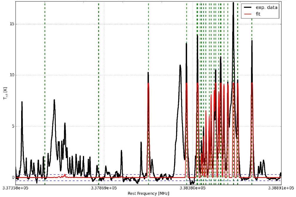
Fig. 8 Result of a single molecule fit for CH\(_3\)OH (continuum subtracted) together with the observed data (continuum subtracted). The horizontal green dotted lines indicate the transition frequencies of CH\(_3\)OH, respectively.
Overall fit
After finishing all single molecule fits for all frequency ranges, the
LineIdentification function performs an overall fit with all
identified molecules, where all frequency ranges are fitted
simultaneously. For this overall fit, the LineIdentification
function creates a further subdirectory within the current job directory
called all, where all required MAGIX files are stored in. The molfit
file for this overall molfit file is made up by merging all optimized
molfit files of the identified molecules from the single molecule fits.
After the overall fit is done, the LineIdentification function
determines the contribution of each molecule described in the optimized
overall molfit file using the myXCLASS function. For that purpose
the LineIdentification function creates a subdirectory within the
all subdirectory called final_fit, which describe the spectrum of
each molecule for each frequency range using the myXCLASS function,
creates a plot showing the (continuum subtracted) observational data
together with the (continuum subtracted) modeled spectrum of a certain
molecule, and stores this plot file in a further subdirectory named with
the name of the current molecule within the final_fit directory.
The name of the plot file is made up of the name of the molecule, the name of the observational data file and the lowest frequency (in MHz) of the corresponding frequency range. The plots for each molecule contribution contain one or more vertical green dotted lines indicating the transition frequencies stored in the database for the corresponding molecule in the given frequency range, see Fig. 9. In addition the horizontal blue dotted line(s) indicate(s) the band of noise, as described above.

Fig. 9 Example of a plot showing the contribution of a single molecule (here \(^{13}\)CH\(_3\)OH\(_{v=0}\)) after finishing the overall fit. The vertical green dotted lines indicate the transition frequencies in the database in the given frequency range.