XCLASS-GUI
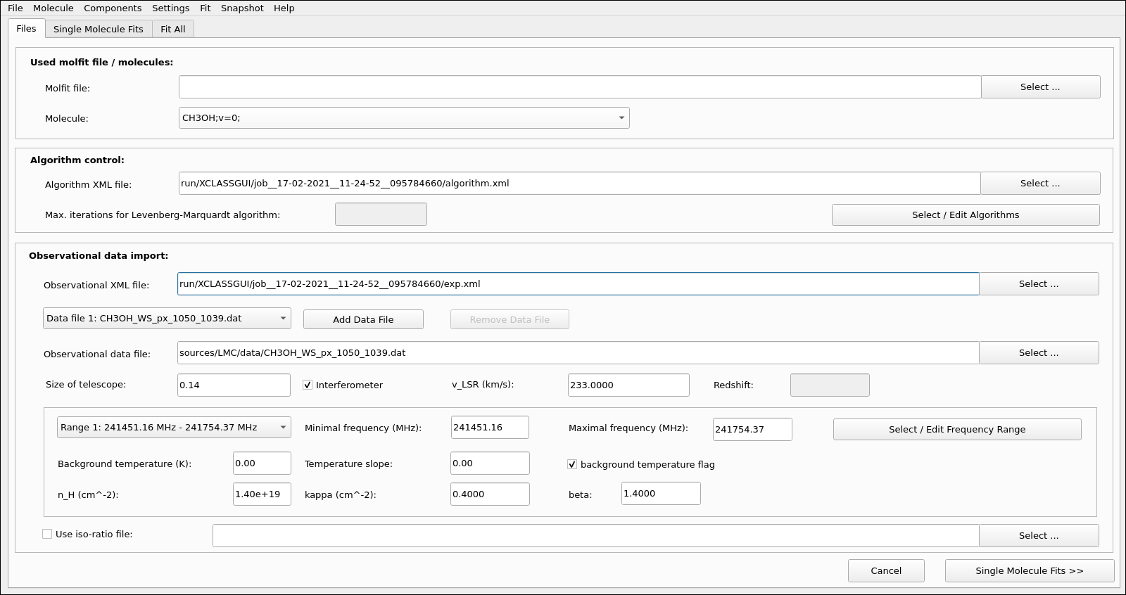
Fig. 10 XCLASS-GUI, Tab: Files.
The XCLASS-GUI can be started at the command line with
XCLASS-GUI --molfit=. --alg=. --obs=.
where the command line arguments molfit
(Sect. “The molfit file”), alg
(Sect. “Algorithm xml file”), and obs
(Sect. “Observational xml file”) are optional and define the path
and name of a molfit, algorithm xml, and obs. xml file, respectively.
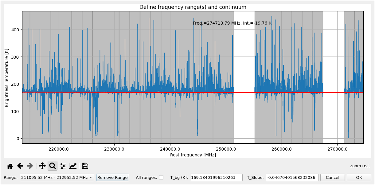
Fig. 11 XCLASS-GUI, Tab: Select Range.
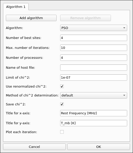
Fig. 12 XCLASS-GUI, Tab: Optimization algorithms.
The graphical user interface (GUI) included in the extended XCLASS package offers the possibility to interactively model observational data and to describe molecules and recombination lines in LTE. It can be used to describe molecular emission and generate synthetic spectra from input physical parameters. These synthetic spectra can be overlaid on the observed spectra and/or fitted to the observations to obtain the best fit to the physical parameters.
The GUI consists of three tabs, where the first tab, see Fig. 10, specifies, among other things, which ranges of the observation data are to be fitted. Here, the definition of the different fitting ranges can be done interactively, see Fig. 11, together with the specification of the corresponding continuum level according to Eq. (21). Additionally, a user friendly GUI interface, see Fig. 12, provides the opportunity to select and control an optimization algorithm used for fitting. Here, different optimization algorithms can be combined to utilize the advantages of different algorithms.
The second tab, see Fig. 13, allows the user to model the contribution of a particular molecule, assessing the effects of changing the input parameters in real time. Here, the synthetic spectra are shown together with the observational data around selected transitions of a certain molecule. Additionally, the molecular parameters for each transitions are displayed as well. Other transitions are available via the arrow buttons. The different transitions can be ordered in four different ways: In ascending order by the energy of the lower state \((E_{\rm low})\), by descending order of the transition strength, i.e. by the product of Einstein A coefficient and upper state degeneracy \((g \cdot A)\), by a weighting factor \(w_j\) defined as
where \(g_j\), \(A_j\) and \(E_{{\rm low}, j}\) represents the upper state degeneracy, the Einstein A coefficient, and the energy of the lower state of a transition \(j\), respectively, and by the transition frequency. In addition to that the user can declare a lower limit for the transition strength, an upper limit for the lower energy, and for the total number of transitions. In the bottom half of the GUI, the LTE parameters for a certain molecule and component are shown. Here, the user can define ranges for each parameter and component, add or remove components, and activate or deactivate the contribution of a certain component to the synthetic spectra to estimate the contribution of a certain component. Finally, the physical parameters for the current molecule can be fitted directly to the observational data using the optimization algorithm(s) defined in the previous tab. Here, individual parameters can be fixed as well.

Fig. 13 XCLASS-GUI, Tab: “Single-Molecule-Fits”
Finally, the third tab, see Fig. 14, displays the synthetic spectra including the contributions of all molecules together with the observational data. Additionally, the parameters for each molecule and component are shown as well. Moreover, the GUI offers the possibility to fit all parameters of all components simultaneously to take line blending effects into account.
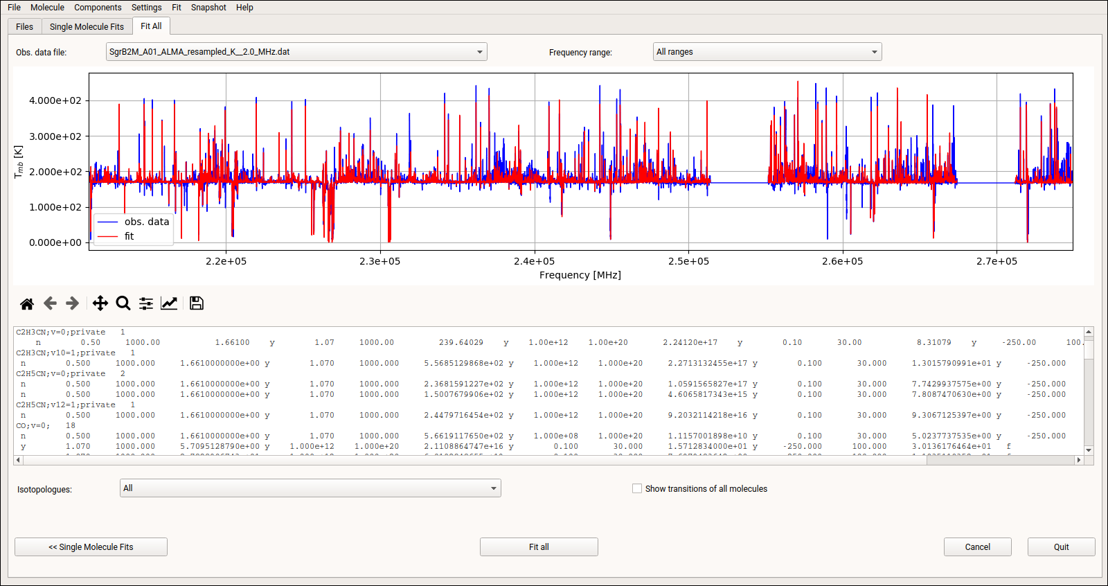
Fig. 14 XCLASS-GUI, Tab: “Fit-All”.